epiinfer-contact-tracing
Tutorial: forecast an epidemic with epiinfer-contact-tracing in Docker
This tutorial takes you from nothing to a forecast, a back-test of how good that forecast is, and a comparison with the paper’s other methods. Everything runs inside the Docker image, so you need nothing installed except Docker.
You will:
- simulate an epidemic in 10,000 people, so that the true outcome is known;
- look at the data;
- forecast 14 days ahead from day 60, then check the forecast against what happened;
- make a genuine forecast past the end of the data;
- back-test: forecast from every day from 25 to 79 and measure the error;
- compare epiinfer-contact-tracing (both engines) with the earlier EpiInfer, ARIMA and Holt-Winters;
- convert your own case and contact lists, and forecast with them.
Time: about 10 minutes. Step 6’s 2025-engine back-test is about 7 of them.
Same numbers as here. Steps 1–6 are
docs/tutorial/run_tutorial.sh, and every table and plot in them
is that script’s output (the files are in
docs/tutorial/outputs and
docs/tutorial/img). CI runs the script inside the Docker image on every
change and fails if any number differs, so you should get exactly these results. All the
randomness is seeded.
The numbers were checked on two platforms: the Docker image on Linux (Intel/AMD) and a native run on an Apple-silicon Mac:
- Both epiinfer-contact-tracing engines: bit-identical.
- The earlier EpiInfer and ARIMA: equal to better than one part in a billion (last-digit rounding).
- Holt-Winters: differs by up to 0.2%, because its statsmodels fit is platform-sensitive.
- The plots: can differ in font rendering.
0. Set up
Install Docker
- macOS or Windows: install Docker Desktop and start it.
- Linux: install Docker Engine.
Check it works:
docker --version
Get the image
Pull the released image (it works on Intel/AMD and ARM, including Apple silicon):
docker pull ghcr.io/nuzla/epitrace:0.3.0
Or build it from a checkout of this repository:
git clone https://github.com/nuzla/epitrace.git
cd epitrace
docker build -f docker/Dockerfile -t ghcr.io/nuzla/epitrace:0.3.0 .
Make a working folder and a shortcut
mkdir -p epitrace-tutorial/data epitrace-tutorial/results
cd epitrace-tutorial
The shell function epi runs one epitrace command in a fresh container:
epi() { docker run --rm --user "$(id -u):$(id -g)" \
          -v "$PWD/data:/data" -v "$PWD/results:/work/results" \
          ghcr.io/nuzla/epitrace:0.3.0 "$@"; }
How the pieces fit together:
| On your computer | Inside the container | What goes there |
|---|---|---|
./data |
/data |
datasets |
./results |
/work/results (the working directory) |
everything the commands write |
- Paths. Arguments are container paths: datasets are
/data/...and outputs areresults/.... --user "$(id -u):$(id -g)"makes the files the container writes belong to you.- Windows. Run the commands in WSL or Git Bash.
Check the shortcut:
epi --version
epitrace 0.3.0
1. Simulate an epidemic
To judge a forecast you need to know what really happened. So we first simulate an epidemic with the paper’s agent-based model, AgeMixABM:
epi simulate --out /data/my_epidemic --contact age_structured --days 100 --seed 123
This takes a few seconds and writes data/my_epidemic/.
The simulated population:
- People. 10,000, in three age groups: 2,455 aged 0–19, 5,422 aged 20–60 and 2,123 aged 61+.
- Contacts. Each day people meet according to an age-structured contact matrix. 70% of first-day contacts recur every day; the rest are re-drawn daily. Symptomatic people make no contacts (they isolate).
- Disease. A contact with a pre-symptomatic person (A) infects with probability p1. After 7 days in A, a person becomes symptomatic (I) with probability p2; otherwise they return to susceptible (S). Symptomatic people recover (R) after 7 days and become susceptible again 7 days later.
-
True rates. They differ by age group:
Age group p1 p2 0–19 0.25 0.15 20–60 0.15 0.10 61+ 0.08 0.05
The folder holds the files described in DATA_FORMAT.md:
| File | Content |
|---|---|
individual_day_state.csv |
every person’s state (0 = S, 1 = A, 2 = I, 3 = R) on every day |
timed_edges.csv |
every contact: day, person i, person j |
states_total.csv |
daily totals of S, A, I, R |
age_group_population.csv |
group sizes |
daily_group_infected.csv, daily_group_avg_contacts.csv |
daily counts per age group |
The forecast target throughout is the number of symptomatic people, I.
2. Look at the data
epi describe --data /data/my_epidemic --plot results/01_epidemic_curve.png
dataset            my_epidemic
people             10000
days               0-100
peak symptomatic   919 on day 19
contacts per day   34187 (days 1-100)
pre-symptomatic A  recorded
usable engines     final, contact, compartmental
results/01_epidemic_curve.png
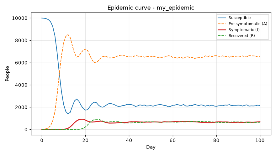
- The shape. The epidemic peaks at 919 symptomatic people on day 19. Because immunity lasts only 7 days, it then settles at about 650–700 symptomatic people a day.
- Why A is so large. Most people are in A at any moment, because only 5–15% of infections ever become symptomatic.
- Usable engines. This line lists which of the library’s three methods can run on the
folder:
final: the October 2026 epiinfer-contact-tracing. It needs only who is symptomatic or recovered, plus the contacts.contact: the 2025 epiinfer-contact-tracing. It also needs who is in A, which only simulations record.compartmental: the earlier EpiInfer. It needs only daily counts per age group.
3. Forecast from day 60
Pretend it is day 60: forecast the next 14 days, using nothing after day 60. Because the data continue to day 100, we can then see how close the forecast came.
epi forecast --data /data/my_epidemic --from-day 60 --horizon 14 \
  --out results/02_forecast_day60.csv --plot results/02_forecast_day60.png
What the default (final) engine does:
- Calibrate. It searches a grid of p1 and p2 values (0.05–0.30) for the pair whose
7-day forecasts best matched the last 14 days. This is method
unknown_both, the default: neither rate is given. It uses one (p1, p2) for everyone. - Rebuild the pre-symptomatic people. It infers them from who became symptomatic: each symptomatic person stands for 1/p2 exposures, and the unseen ones are drawn from the people who had contacts. It never reads state A, which real data would not have.
- Simulate. It runs 30 simulated futures on the day-60 contact network and reports their mean and 10th–90th percentiles.
results/02_forecast_day60.csv:
group,origin_day,target_day,horizon,mean,p10,p90,actual,p1_used,p2_used
ALL,60,61,1,688.7,678.0,699.0,700.0,0.125,0.1
ALL,60,62,2,679.6,661.6,691.5,709.0,0.125,0.1
ALL,60,63,3,648.9,628.8,662.0,684.0,0.125,0.1
ALL,60,64,4,670.2,647.7,693.2,708.0,0.125,0.1
ALL,60,65,5,663.6333333333333,641.0,682.3,715.0,0.125,0.1
ALL,60,66,6,660.0666666666667,635.0,684.9,713.0,0.125,0.1
ALL,60,67,7,632.9333333333333,603.8,656.2,701.0,0.125,0.1
ALL,60,68,8,637.0333333333333,614.8,654.5,694.0,0.125,0.1
ALL,60,69,9,643.3333333333334,617.4,665.0,696.0,0.125,0.1
ALL,60,70,10,643.2666666666667,611.2,667.3,691.0,0.125,0.1
ALL,60,71,11,635.6,612.8,661.0,677.0,0.125,0.1
ALL,60,72,12,636.7666666666667,607.7,666.0,657.0,0.125,0.1
ALL,60,73,13,643.2333333333333,609.4,677.3,648.0,0.125,0.1
ALL,60,74,14,644.2,612.0,674.4,627.0,0.125,0.1
| Column | Meaning |
|---|---|
origin_day |
the last day the forecast could see |
target_day, horizon |
the day forecast, and how many days ahead it is |
mean, p10, p90 |
the forecast: the average of the 30 simulated futures, and their 10th and 90th percentiles |
actual |
what really happened (empty for days beyond the data) |
p1_used, p2_used |
the calibrated rates |
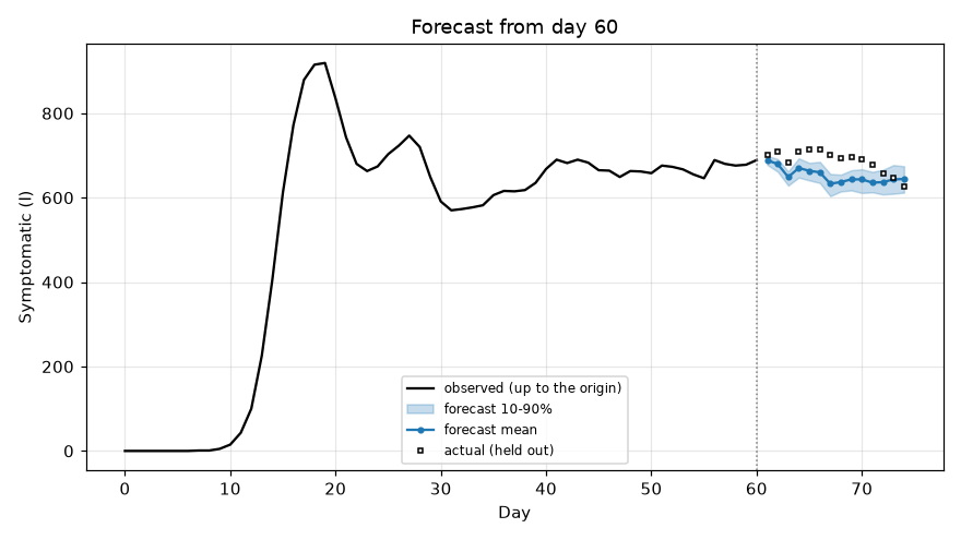
Reading the result:
- The rates. Calibration chose p1 = 0.125 and p2 = 0.10, close to the adults’ true values (0.15, 0.10). Adults are more than half the population.
- The forecast. It follows the level of the epidemic but runs 5–10% low on days 64–71. The true count is inside the 10–90% band only on days 72–74. The band is narrow because the thirty simulations capture the randomness of the epidemic, not the uncertainty in the calibrated rates.
4. Forecast past the end of the data
Leave out --from-day and the forecast starts from the last observed day, 100:
epi forecast --data /data/my_epidemic --horizon 14 \
  --out results/03_forecast_future.csv --plot results/03_forecast_future.png
group,origin_day,target_day,horizon,mean,p10,p90,actual,p1_used,p2_used
ALL,100,101,1,675.0,664.9,683.1,,0.125,0.1
ALL,100,102,2,673.0666666666667,659.9,689.0,,0.125,0.1
...
ALL,100,114,14,644.3333333333334,616.8,668.5,,0.125,0.1
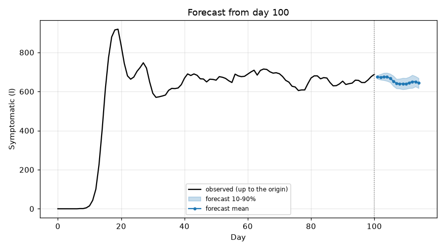
This is what you would do with live data. actual is empty because those days have not
happened. Contacts after day 100 are unknown, so day 100’s network is reused for every
future day.
5. Back-test: how good are the forecasts?
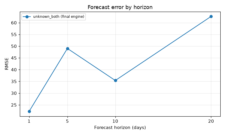
One forecast tells you little. A back-test forecasts from every day in turn, here every day from 25 to 79, using only the data up to that day. It then scores the forecasts made 1, 5, 10 and 20 days ahead against the truth.
epi run --data /data/my_epidemic --method unknown_both \
  --out results/04_backtest_final --plots
    dataset       method group  horizon  n      rmse    frmse  frmse_rel
my_epidemic unknown_both   ALL        1 55 22.196007 0.033632   0.035648
my_epidemic unknown_both   ALL        5 55 49.020250 0.074571   0.078426
my_epidemic unknown_both   ALL       10 55 35.380628 0.053350   0.053851
my_epidemic unknown_both   ALL       20 55 62.659970 0.094455   0.091550
results/04_backtest_final/forecast_my_epidemic_unknown_both.png
results/04_backtest_final/rmse_my_epidemic_unknown_both.png
| Column | Meaning |
|---|---|
n |
number of forecasts scored (55 origins, days 25–79) |
rmse |
root mean squared error, in people |
frmse |
RMSE divided by the mean actual count (the paper’s 2025 “fractional RMSE”) |
frmse_rel |
root mean squared relative error (the October 2026 paper’s fRMSE) |
A 1-day forecast is off by about 22 people out of roughly 660, or 3–4%. Twenty days ahead the error is about 63 people, or 9%.

Each panel plots, for one horizon, every forecast (blue, dashed) against what happened (grey) on the day it was aimed at.
Files in results/04_backtest_final/:
| File | Content |
|---|---|
predictions_my_epidemic_unknown_both.csv |
every forecast: origin, target day, predicted, actual, rates used |
rates_my_epidemic_unknown_both.csv |
the (p1, p2) in use at each origin |
summary_my_epidemic_unknown_both.csv |
the table above |
The rates are recalibrated every 5 days and damped (a new estimate replaces the old one only as far as it fits better). They start at (0.15, 0.10). They drift to (0.10, 0.12) by day 75 as the epidemic settles.
6. Compare with the paper’s other methods
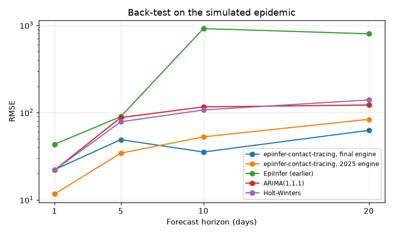
The paper compares epiinfer-contact-tracing (which it calls EpiInfer-contact) with the earlier EpiInfer, ARIMA, Holt-Winters and an LSTM. The library has all but the LSTM. All of the following use the same forecast origins (25–79).
6a. epiinfer-contact-tracing, 2025 engine
epi run --data /data/my_epidemic --engine contact --method unknown_both \
  --horizons 1 5 10 20 --last-origin 79 --out results/05_backtest_contact
This is the code behind most of the paper’s tables. It calibrates a separate (p1, p2) for each age group every day, and forecasts each group. It is seeded with the true list of pre-symptomatic people from the simulator, an advantage real data cannot give. It prints a row per age group plus the total; the totals are:
    dataset       method group  horizon  n      rmse    frmse  frmse_rel
my_epidemic unknown_both   ALL        1 55 11.684699 0.017705   0.018046
my_epidemic unknown_both   ALL        5 55 34.310136 0.052194   0.055401
my_epidemic unknown_both   ALL       10 55 52.779822 0.079586   0.083180
my_epidemic unknown_both   ALL       20 55 83.813474 0.126343   0.123363
This back-test takes about 7 minutes.
6b. The earlier EpiInfer
epi run --data /data/my_epidemic --engine compartmental --method unknown_both \
  --out results/06_backtest_compartmental
    dataset       method group  horizon  n       rmse    frmse  frmse_rel
my_epidemic unknown_both   ALL        1 55  43.414112 0.065783   0.066390
my_epidemic unknown_both   ALL        5 55  89.916927 0.136784   0.147207
my_epidemic unknown_both   ALL       10 55 917.458551 1.383419   1.407327
my_epidemic unknown_both   ALL       20 55 800.591472 1.206834   1.213571
This is the authors’ previous model. It is a deterministic compartmental model that uses only daily counts per age group, with no contact list, and it takes under a second.
With both rates unknown it fits p1 and p2 to the last five days only. On this epidemic the fit puts p2 at the top of the grid (0.30, three times the true adult value) at 75% of the origins, so forecasts 10–20 days ahead overshoot badly. The paper’s own tables show the same pattern for this model.
6c. Statistical baselines
epi baseline --data /data/my_epidemic --which arima --last-origin 79 --out results/07_arima.csv
epi baseline --data /data/my_epidemic --which holt_winters --last-origin 79 \
  --out results/07_holt_winters.csv
method  horizon  n       rmse    frmse
 arima        1 55  21.966988 0.033285
 arima        5 55  87.692891 0.133401
 arima       10 55 116.345709 0.175436
 arima       20 55 122.322350 0.184392

      method  horizon  n       rmse    frmse
holt_winters        1 55  21.985009 0.033312
holt_winters        5 55  78.473990 0.119377
holt_winters       10 55 107.270618 0.161751
holt_winters       20 55 139.720527 0.210619
Both use only the daily count of symptomatic people:
- ARIMA(1,1,1) is refitted on the whole history at each origin.
- Holt-Winters (additive damped trend) is refitted on the last 14 days.
6d. Everything on one chart
epi plot-rmse \
  "epiinfer-contact-tracing, final engine=results/04_backtest_final/summary_my_epidemic_unknown_both.csv" \
  "epiinfer-contact-tracing, 2025 engine=results/05_backtest_contact/summary_my_epidemic_unknown_both.csv" \
  "EpiInfer (earlier)=results/06_backtest_compartmental/summary_my_epidemic_unknown_both.csv" \
  "ARIMA(1,1,1)=results/07_arima.csv" \
  "Holt-Winters=results/07_holt_winters.csv" \
  --out results/08_rmse_comparison.png --title "Back-test on the simulated epidemic" --log-y
| RMSE (people) | 1 day | 5 days | 10 days | 20 days |
|---|---|---|---|---|
| epiinfer-contact-tracing, final engine | 22.2 | 49.0 | 35.4 | 62.7 |
| epiinfer-contact-tracing, 2025 engine (uses the true A) | 11.7 | 34.3 | 52.8 | 83.8 |
| EpiInfer, earlier model | 43.4 | 89.9 | 917.5 | 800.6 |
| ARIMA(1,1,1) | 22.0 | 87.7 | 116.3 | 122.3 |
| Holt-Winters | 22.0 | 78.5 | 107.3 | 139.7 |
What this shows, for this one epidemic and seed:
- Up to 5 days, the 2025 engine is best, helped by knowing who is pre-symptomatic.
- At 10 and 20 days the final engine is best, without that information.
- From day 5 on, both epiinfer-contact-tracing engines beat ARIMA and Holt-Winters. At day 1 the final engine and the baselines tie (22 people): a day ahead, “tomorrow ≈ today” is hard to beat.
- The earlier EpiInfer, with both rates unknown, is the least accurate.
- Noise. One simulated epidemic gives one sample. Differences of a few people are within
Monte-Carlo noise: add
--seed 1,--seed 2… to theruncommands to see how much results vary.
7. Your own data
The files
The default engine needs only two things for each day:
- who is symptomatic or recovered, in
individual_day_state.csv; - who met whom, in
timed_edges.csv.
data/my_data/
  individual_day_state.csv     id,day,state      (2 = symptomatic, 3 = recovered, else 0)
  timed_edges.csv              day,i,j
  age_group_population.csv     age_group,population     (gives the population size)
People are numbered 0 … N−1 and days 0, 1, 2 … The full specification is in DATA_FORMAT.md.
Convert a case list and a contact list
Most contact-tracing systems keep a list of cases (who, and the date symptoms began) and a list of contacts (date, person, person):
cases.csv                 contacts.csv
person,onset              date,a,b
P1,2026-05-12             2026-03-02,P6230,P8047
P2,2026-03-24             2026-03-02,P4062,P8490
...                       ...
epitrace from-cases turns them into a dataset folder. Each case is symptomatic for
--duration days from onset and recovered (immune) for --rec-duration days after that:
cp /path/to/cases.csv /path/to/contacts.csv data/
epi from-cases --cases /data/cases.csv --contacts /data/contacts.csv --out /data/my_data \
  --duration 7 --rec-duration 7
wrote /data/my_data: 9981 people, days 0-99 (day 0 = 2026-03-02)
Person labels can be any text; people.csv in the output maps the numeric ids back to
them. In Python the same is epitrace.convert.cases_to_dataset, and
examples/convert_case_list.py
is a script version.
The output above comes from the tutorial epidemic written out as a case list and a contact
list. Starting from just those two files, describe sees the same epidemic, now without
state A:
dataset            my_data
people             9981
days               0-99
peak symptomatic   919 on day 18
contacts per day   34187 (days 0-99)
pre-symptomatic A  not recorded
usable engines     final
(The 19 people who never had a contact or symptoms are not in the files, and day 0 is now the first contact day, so day numbers are one lower than in the simulation.)
Forecast
epi describe --data /data/my_data
epi forecast --data /data/my_data --horizon 14 --duration 7 --rec-duration 7 \
  --out results/my_forecast.csv --plot results/my_forecast.png
epi run --data /data/my_data --method unknown_both --duration 7 --rec-duration 7 \
  --out results/my_backtest --plots
Settings that matter
| Option | Meaning | Default |
|---|---|---|
--inc |
days infected before symptoms | 7 |
--duration |
days symptomatic | 7 |
--rec-duration |
days immune after recovery before reinfection is possible (final engine) | 7 |
--method |
which rates you know: unknown_both, known_p1, known_p2, known_both (with --p1-true / --p2-true) |
unknown_both |
--engine |
final, contact (needs state A) or compartmental (needs the per-group count files) |
final |
--seed, --num-sims |
random seed; simulated futures per forecast | 0; 30 |
--start-eval, --last-origin, --horizons |
back-test origins and horizons | 25; 79; 1 5 10 20 |
--max-day |
run only: use the days up to this one. Raise it (with --last-origin) to back-test data longer than 100 days; forecast always uses every day |
100 |
Set --inc, --duration and --rec-duration to what is known about your disease. The
model does not estimate them.
Aggregate data only? If you have daily counts per age group but no individual records or
contacts, use --engine compartmental. It needs states_total.csv,
age_group_population.csv, daily_group_infected.csv and daily_group_avg_contacts.csv.
8. Reproducing the paper’s tables
With the paper’s datasets in ./data (see REPRODUCING.md for where they
come from and what each table needs):
epi reproduce --table epiinfer_age_structured --data /data/age_structured --out results/paper
epi reproduce --table appendix --scale 0.2 --data /data/appendix_april0.2 --jobs 4 --out results/paper
epi reproduce --table openabm --data /data/openabm --out results/paper
The first takes under a second and reproduces the earlier EpiInfer’s row of Tables 2–5 and 14 exactly:
                    table     method  horizon contacts  paper_rmse    rmse  rmse_ratio  paper_frmse  frmse  n_origins
Tables 2-5, 14 (EpiInfer) known_both        1 same_day     180.172 180.172       1.000        0.262  0.262         61
Tables 2-5, 14 (EpiInfer) known_both        5 same_day     408.346 408.346       1.000        0.597  0.597         61
Tables 2-5, 14 (EpiInfer) known_both       10 same_day     161.629 161.629       1.000        0.243  0.243         61
Tables 2-5, 14 (EpiInfer) known_both       20 same_day      95.961  95.961       1.000        0.143  0.143         61
What reproduces and what does not, and why, is in PAPER_VS_CODE.md.
Apptainer / Singularity
On a cluster without Docker, convert the image once and replace epi with:
apptainer pull epitrace.sif docker://ghcr.io/nuzla/epitrace:0.3.0
epi() { apptainer run --bind "$PWD/data:/data" epitrace.sif "$@"; }
Run from the folder that holds data/ and results/. Apptainer runs as you, so there is no
--user. This route has not been tested by the maintainers.
Troubleshooting
Unable to find image. Run thedocker pull(ordocker build) in step 0 first.Permission deniedwritingresults/. Createresults/before the first run and keep the--user "$(id -u):$(id -g)"part ofepi.dataset folder not found. Give the container path (/data/...), not the path on your computer.from_day must be between .... Calibration needs at least 22 observed days (both rates unknown) before the forecast origin.the first forecast origin must be day 22 or later. The same limit forrun: use--start-eval 22or higher (25 is the default).no forecast could be scored. The data is too short for the--start-evaland--horizonsyou gave.describeshows how many days it has.- Numbers differ from this page. Check
epi --versionsays 0.3.0 and that you kept--seed 123forsimulate. CI compares every number on this page with the image on every change. - Slow. The 2025 engine’s back-test is the slow step (minutes). Give Docker Desktop
more CPUs, or add
--workers 4to run its simulations in threads (results are identical).